Algorithm
Table of Contents
- 1. Basics
- 2. Sorting algorithms
- 3. Data structure
- 4. Trees
- 5. Graph
- 6. TODO String algorithms
- 7. TODO Dynamic Programming
- 8. Other Named Algorithm
- 9. TODO NP-Completeness
- 10. TODO Linear Programming (LP)
- 11. Tips
- 12. Old Writings
1 Basics
1.1 Order of growth
In this section, ∃ c1,c2,n0 means there exists positive constants c1, c2, and n0.
- \(\Theta (g(n))\): "big-theta" of g of n, both lower bound and upper bound, asymptotically tight bound
- O: big-o (most often used), upper bound, asymptotic upper bound
- \(\Omega\): big omega, lower bound, asymptotic lower bound
- o: little-o, not tight upper bound
- \(\omega\): little omega, not tight lower bound
Formally:
- \(\Theta(g(n)) = {f(n) : \exists c_1, c_2, n_0 \text{ such that } 0 \le c_1 g(n) \le f(n) \le c_2 g(n) \text{ for all } n \ge n_0}\)
- O(g(n)) = {f(n): ∃ c and n0 such that 0 ≤ f(n) ≤ c g(n) for all n ≥ n0}
- Ω(g(n)) = {f(n): ∃ c and n0 such that 0 ≤ c g(n) ≤ f(n) for all n ≥ n0}
- o(g(n)) = {f(n): ∃ c and n0 such that 0 ≤ f(n) < c g(n) for all n ≥ n0}
- ω(g(n)) = {f(n): ∃ c and n0 such that 0 ≤ c g(n) < f(n) for all n ≥ n0}
1.2 TODO how to analyze the running time
1.3 TODO Amortized Analysis
2 Sorting algorithms
| algorithm | worst-case | average case | memory |
|---|---|---|---|
| insertion sort | n2 | ||
| merge sort | n log n | ||
| heap sort | n log n | in place | |
| quick sort | n2 | n log n | |
| counting sort | n+k | ||
| radix sort | d(n+k) | ||
| bucket sort | n2 | n |
2.1 Bubble sort
Go through the array n items. Each time, swap two adjacent items a and b if a>b. Each loop, the largest one go to the end, the smaller ones bubbles up.
for i in range(n):
  for j in range(n-i):
    if A[j] > A[j+1]:
      swap(A[j], A[j+1])
2.2 insertion sort
Each loop, make sure the first i items are sorted. In the i-th loop, insert the i-th item into the correct position.
for i in 1 to A.length:
  key = A[i]
  j = i-1
  while A[j] > key:
    A[j+1] = A[j]
    j--
  A[j]=key
2.3 merge sort
Uses divide-and-conquer, recursively solve the left and right subarray, and merge the two sorted arrays (in linear time).
def sort(A, p, r):
  if p < r:
    q = (p + r) / 2
    sort(A, p, q)
    sort(A, q, r)
    merge(A, p, q, r)

def merge(A, p, q, r):
  n = q-r+1
  L = A[p:q]
  R = A[q:r]
  l = r = 0
  for i in range(n):
    if L[l] < R[r]:
      A[i] = L[l]
      l++
    else:
      A[i] = R[r]
      r++
2.4 Heap sort
Binary heap is a nearly complete binary tree, i.e. completely filled on all levels except possibly the lowest, which is filled from left up to a point. It can be either max-heap or min-heap, with the max and min on top of heap respectively.
Some helper routines:
def parent(i):
  return floor(i/2)
def left(i):
  return 2*i
def right(i):
  return 2*i+1
Assuming the trees rooted at left(i) and right(i) are max-heaps,
but A[i] is not. Float down A[i] so that the tree rooted at i is
max-heap.
def max_heapify(A, i):
  l = left(i)
  r = right(i)
  # TODO check l,r < A.heap_size
  value, index = max(A[i], A[l], A[r])
  if index != i:
    swap(A[i], A[index])
    max_heapify(A, index)
Build a heap from an array:
def build_max_heap(A):
  for i in range(len(A), 1, -1):
    max_heapify(A, i)
Finally heap sort: in each loop, remove the top (current max item),
replace it with the last element in the heap, and do heapify.
def heapsort(A):
  build_max_heap(A)
  for i in range(len(A), 2, -1):
    swap(A[1], A[i])
    A.heap_size--
    max_heapify(A, 1)
2.5 Quick sort
The worst running time is \(\Theta(n^2)\), but it is often the best practical choice for sorting, because it has average running time of \(\Theta(n log n)\), with a small constant factor.
It is an divide-n-conquer algorithm.
- First find a pivot value \(x\), which is typically the last element in the array.
- Then partition the array into two parts, less than \(x\) and larger than \(x\).
- recursively do this for the two partitions
def sort(A):
  quicksort(A, 1, len(A))
def quicksort(A, p, r):
  q = partition(A, p, r)
  quicksort(A, p, q-1)
  quicksort(A, q+1, r)
The partition function:
def partition(A, p, r):
  x = A[r]
  i = p-1
  for j in range(p, r):
    if A[j] <= x:
      i = i+1
      # values less than x swapped to left part
      swap(A[i], A[j])
  # put the pivot value in place
  swap(A[i+1], A[r])
  return i+1
Or I prefer a functional way, in which case we don't even need to
specify the implementation of partition function, as it is obvious:
def quicksort(A):
  x = A[-1]
  Al, Ar = partition(A, x)
  return [quicksort(Al), x, quicksort(Ar)]
2.6 Linear time sorting
All sorting algorithms above are comparison sorts, which can be proved to take at least \(n log n\) running time. The algorithms in this section makes certain assumptions to the array.
2.6.1 couting sort
Assume each of the elements are integers, in the range of [0,k].
The idea:
- maintain an array C[0..k], where C[i] is the number of value
iin A - change the array C such that C[i] is the number of values less than
or equal to
i - put the elements directly to the place according to C
2.6.2 TODO Radix sort
2.6.3 TODO Bucket sort
Assume the input is drawn from a uniform distribution. The average running time is linear.
3 Data structure
This section is mostly empty, because these are obvious. Most important aspects of these data structures are the implementation of their operations.
3.1 linked list
- linked list
- head
- tail
- next
- doubly linked list
- next
- prev
3.2 stack & queue
- push
- pop
- enqueue
- dequeue
3.2.1 [A] priority queue
It is implemented using a heap. Each item has a value. The dequeue
operation makes sure the popped item is the max one or min one, for
max-priority queue and min-priority queue, respectively.
3.3 hash table
4 Trees
4.1 [A] Search
Using binary tree as example. &
BFS:
q = queue()
def traverse(root):
  q.insert(root)
  while (x = q.pop()):
    q.insert(x.children)
    visit(x)
DFS:
traverse(root)

def traverse(node):
  traverse(node.left)
  traverse(node.right)
4.2 [A] Traversal
Only defined for DFS.
Pre-order:
def traverse(node):
  visit(node)
  traverse(node.left)
  traverse(node.right)
In-order (only defined for binary tree):
def traverse(node):
  traverse(node.left)
  visit(node)
  traverse(node.right)
Post-order:
def traverse(node):
  traverse(node.left)
  traverse(node.right)
  visit(node)
4.3 Special Trees
4.3.1 Binary search tree
The value of a node is larger than all values in its left subtree, but smaller than all values in the right subtree. As the name suggested, it is mostly used for searching a value.
4.3.2 red-black tree
A problem of search tree is that, the height may be very large, and the running time is tight with the height.
The red-black tree is a binary search tree. It is designed to be a balanced binary search tree, and guarantees that a simple path from root to any leaf is no more than twice as long as any other, so that the tree is approximately balanced.
Specifically, the property of a red-black tree:
- every node is either red or black
- the root is black
- every leaf is black
- if a node is red, both its children are black
- for each node, all simple paths from the node to leaves contains the same number of black nodes
Operations:
- rotation
- insertion
- deletion
4.3.3 interval tree
This is an example of augmenting data structures. It is an augmented red-black tree. Each node of a tree contains two additional attributes: the low and high of the sub-tree. Thus it is easier for search, as we can use the interval to decide whether the subtree contains the value at all.
4.3.4 B-tree
B-tree is a balanced search tree, designed to work well on storage devices. B-tree is not a binary tree.
Specifically, a B-tree is defined as:
- each node contains n keys, where \(t \le n \le 2t-1\), and contains \(n+1\) children.
- similar to binary search tree, the children of a node is divided by the keys, i.e. $ch1 ≤ key1 ≤ ch2 ≤ key2 …$.
- All leaves have the same depth
The operations:
- search: obvious
- insertion: this is tricky. Since each tree node has a capacity of \([t,2t-1]\), when a node is full, it must be split, and a new key needs to be generated.
- deletion: this is also tricky, as when the node is filled with less than \(t\), it must be merged.
4.3.5 prefix-tree
The prefix tree, also called Trie, digital tree, radix tree, is one kind of search tree, in which all descendants of a node share a common prefix.
4.4 Heap
4.4.1 TODO Fibonacci Heap
5 Graph
The representation of a graph can be either a adjacent list or adjacent matrix.
A graph is (V,E), each edge has a weight.
Some general notations:
- A cut of an undirected graph G is a partition of V, into \((S, V-S)\).
- An edge E crosses the cut if its two ends belong to the different sides of the cut.
- A cut respects a set of edges A if no edge in A crosses the cut
- The minimum weight edge crossing the cut is called light edge
- More generally, we say an edge the light edge for some properties, if it is the minimum weight one among all edges satisfying the property.
5.1 DFS & BFS
Same as trees, except checking for repeat (by coloring).
5.2 topological sort
Run DFS (or BFS) and print out the nodes.
5.3 Minimum Spanning Tree
Given a graph (V,E), and each edge has a weight. Find the subset of edges \(E' \subset E\) such that (V,E') is a tree. This tree is called spanning tree. The spanning tree with minimum sum of edge weights is called the minimum spanning tree.
General idea: We grow a set of edges A, from \(\emptyset\), and maintain the invariant that is a subset of some minimum spanning tree. If we can add an edge to A, and don't violate this invariant, we call it safe edge to A.
A = {}
while A is not a spanning tree:
  find (u,v) that is safe for A
  A = A union {(u,v)}
Theorem 23.1:
\(A\) is a subset of \(E\), and \(A\) is in some minimum spanning tree of G. Cut \(c\) respects A. Then the light edge of \(c\) is safe to \(A\).
Corollary 23.2
A is a subset of E and A is included in some minimum spanning tree of G. We have a forest F=(V,A). In the forest, there will be many connected components \(C_i\).
Then the light edge connecting \(C_i\) to \(C_j\) is safe to A.
5.3.1 Kruskal's algorithm
This algorithm grow the edges, or forest. It sorts all edges. Starting from empty, greedily find the smallest edge as long as it does not form a cycle.
edges = sorted(edges, key=weight)
A = {}
for (u,v) in edges:
  if u,v are not in the same component of A:
    add (u,v) to A
5.3.2 Prim's algorithm
This algorithm will grow the tree, i.e. at any given time, the result is a tree. Start from an arbitrary node, add it to A. Each step, add to A the light edge from a node A to the rest of G.
for u in G.V:
  u.key = infinite
  u.parent = None
r = random_node()
Q = G.V
while Q:
  u = extract_min(Q, key=key)
  for v in G.Adj[u]:
    if v in Q and w(u,v) < v.key:
      v.key = w(u,v)
      v.parent = u
5.4 Shortest path
Given a weighted, directed graph, the shortest path from u to v is the path that has minimum weight. We talk mainly about single-source, single-destination shortest path.
We add to attributes to vertices of the graph:
v.d: the upper bound of shortest path from s to v. Initialize to infinite.v.pred: the predecessor for that upper bound. Initialize to nil.
First a helper function, relax of an edge (u,v), by checking whether setting v.pred to u improve v.d:
def relax(u,v):
  if v.d > u.d + w(u,v):
    v.d = u.d + w(u,v)
    v.pred = u
5.4.1 Bellman-Ford algorithm
This is kind of a brute force algorithm. It relax all edges \(|V|-1\) times. Each time, at least one node is set to its optimal, and the source vertex s.d=0, thus \(|V|-1\) iterations will make sure all vertices are set to optimal.
def bellman_ford():
  for i in range(|V|-1):
    for (u,v) in |E|:
      relax(u,v)
The running time is |V||E|
5.4.2 Dijkstra's algorithm
In addition to weighted, directly graph, it assumes all weights are non-negative. The key idea has two fold:
- It maintains a set S of vertices whose "d" has been determined.
- Every iteration, it tries to determine one more vertex. It greedily choose the one with minimum "d".
def dijkstra():
  sovled = {}
  s.d = 0
  q = min_priority_queue(V, "d")
  while q:
    u = q.pop_min()
    solved.insert(u)
    for v in u.adj:
      relax(u,v)
The running time is \(|V|^2 + |E|\). If the priority queue is implemented using Fibonacci heap (TODO), the running time is \(|V| log |V| + |E|\).
5.5 Network Flow Problems
The constraints of a flow network:
- capacity constraint: 0 ≤ f(u,v) ≤ c(u,v)
- flow conservation: ∑v∈ V f(v,u) = ∑v ∈ V f(u,v). I.e. the ingoing and outgoing flow of a node shall equal.
We are interested in two equivalent problems:
- maximum flow
- minimum cut
Residual network:
- Residual network: given capacity c and flow f, the capacity of residual network \(c_f\) is simply \(c(u,v)-f(u,v)\).
- augmenting path: given a flow network G and a flow f, the augmenting path p is a simple path from s to t in the residual network \(G_f\)
The cut of a flow is (S,T) where S + T = V. The flow f(S,T) across the cut is defined as:
\[f(S,T) = \sum_{u\in S} \sum_{v \in T} f(u,v) - \sum_{u\in S} \sum_{v \in T} f(v,u)\]
The capacity of the cut is:
\[c(S,T) = \sum_{u\in S} \sum_{v \in T} c(u,v)\].
The minimum cut is the one whose capacity is minimum. The max-flow min-cut theorem states that the minimum cut equals to the max-flow. Specifically, the following conditions are equivalent:
- f is maximum flow in G
- The residual network \(G_f\) contains no augmenting paths
- |f|=c(S,T) for some cut (S,T) of G.
- This should be further written as |f| equal to the capacity of minimum cut of G.
5.5.1 Ford-Fulkerson method
It is a method instead of an algorithm because it has several different implementations with different running time.
The general ford-fulkerson:
f = 0
while True:
  res_net = residual_network(G, f):
  aug_p = augmenting_path(res_net)
  if not aug_p: break
  do_augment(aug_p)
return f
Apparently the key point is how to find the augmenting path. If chosen poorly, it may not terminate.
5.5.2 Edmonds-Karp algorithm
This algorithm is to use BFS for finding the augmenting path. The shortest path (with unit edge weight) from s to t is selected in this way. It runs in O(VE2), i.e. polynomial time.
6 TODO String algorithms
6.1 TODO Substring matching
6.2 TODO Rabin-Karp algorithm
6.3 TODO Knuth-Morris-Pratt algorithm
7 TODO Dynamic Programming
The core idea is to store the solution to subproblems, thus avoid repeated computation. It uses additional memory to save computation time.
There are often two approaches for dynamic programming:
- Do recursion as usual, but just keep a look up table for each subproblem, i.e. when solving a subproblem, check the table to see if it is already solved, if not, solve it and store its result.
- This is the most commonly used and most efficient algorithm. The above is inefficient by a constant factor. We can order the subproblems based on its size, and the latter subproblems often directly uses the results from the smaller subproblems.
7.1 The rod-cutting problem
Given a rod of length n, and a price table mapping from lengths to prices. Determine the maximum revenue obtainable by cutting and selling the rod.
def cutrod(price_table, n):
  r[0] = 0
  for i in range(1, n):
    q=0
    for j in range(1, i):
      q = max(q, p[i]+r[i-j])
    r[i] = q
return r[n]
7.2 TODO Largest common subsequence
8 Other Named Algorithm
8.1 Bloom Filter
It is used to judge whether an item is in a set or not.
If bloom() return false, it is false. But if bloom() return true, it may not be true.
The basic idea is, hash(item), map it in a vector of m size. The vector is 0 initially. v[hash(item)] is set to 1. To reduce fault rate, use k hash functions.
To verify, only if all k hash functions has 1 in the vector will it return true. Otherwise return false.
9 TODO NP-Completeness
9.1 Approximation algorithms
9.1.1 the vertex-cover problem
9.1.2 the traveling-salesman problem
9.1.3 the set-covering problem
9.1.4 the subset-sum problem
10 TODO Linear Programming (LP)
10.1 Standard and slack forms
10.2 Formulating
10.3 Simplex algorithm
10.4 Duality
11 Tips
11.1 TODO Devide-and-Conquer
11.2 Recursive
11.3 Dynamic Programming
12 Old Writings
12.1 Barrel shifter
A barrel shifter is a digital circuit that can shift a data word by a specified number of bits in one clock cycle.
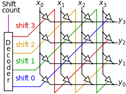
In the above image, x is input and y is output.
For shift 1, all the erjiguan on the green line exist, while others not.
12.1.1 shift register
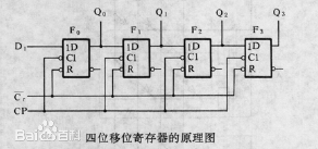
F0、F1、F2、F3是四个边沿触发的D触发器,每个触发器的输出端Q接到右边一个 触发器的输入端D。因为从时钟信号CP的上升沿加到触发器上开始到输出端新状 态稳定地建立起来有一段延迟时间,所以当时钟信号同时加到四个触发器上时, 每个触发器接收的都是左边一个触发器中原来的数据(F0接收的输入数据D1)。寄 存器中的数据依次右移一位。
12.2 Linear congruential generator
A linear congruential generator (LCG) is an algorithm that yields a sequence of pseudo-randomized numbers.
pseudorandom number generator algorithms(PRNG).
\(X_{n+1} = (aX_n+c) mod m\)
X array is the pseudorandom.
- \(X_0\): seed
m: modulusa: multiplierc: increment
If c = 0, the generator is often called a multiplicative congruential generator (MCG), or Lehmer RNG. If c ≠ 0, the method is called a mixed congruential generator.
12.3 Dynamic Programming
Solve problem by breaking down into simpler sub-problems.
12.3.1 One dimension
Given n, find the number of different ways to write n as the sum of 1,3,4
12.3.1.1 Define sub-problems
Dn is the number of ways to write n as sum of 1,3,4
12.3.1.2 Recurrence formula
Dn = Dn-1 + Dn-3 + Dn-4
12.3.2 Two Dimensions
Given two string x and y, find the length of longest common sub-sequence.
12.3.2.1 Define sub-problems
Dij is the length for xi..i and y1..j
12.3.2.2 Recurrence formula
Dij =
- if xi = yi: Di-1,j-1 + 1
- otherwise: max{Di-1,j, Di,j-1}
12.3.3 Interval DP
Given a string x=x1..n, find the minimum number of characters that need to be inserted to make it a palindrome.
12.3.3.1 Define sub-problem
Di,j be the minimum number of characters.
12.3.3.2 Recurrence formula
say y1..k is the palindrome for xi..j, we have either y1 = xi or yk = xj
Dij =
- if xi ≠ xj: 1 + min{Di+1,j, Di,j-1}
- if xi = xj: Di+1,j-1
12.3.4 Tree DP
Given a tree, color nodes black as many as possible without coloring two adjacent nodes.
12.3.4.1 Define
- B(r) as the maximum nodes if the (root) node r is colored black.
- W(r) as the maximum nodes if the (root) node r is colored white.
12.3.4.2 Recurrence
- B(v) = 1 + ∑children W(c)
- W(v) = 1 + ∑children max{B(c), W(c)}
12.4 String Algorithm
12.4.1 Knuth–Morris–Pratt(KMP)
Match a pattern string P inside given long string T.
The idea is, when failure happens, we shift multiple position instead of just 1.
We are able to do that because when the failure happens, we know what have been examined, so we have everything available to make the best choice.
Specifically, we build a look-up table, for the pattern string.
The table has an entry for each index of the string, describing the shift position.
E.g., ABCABDA, the lookup table will be: 0000120.
Actually the table refers to what's the substring matched the prefix of the pattern string.
The algorithm to build the table:
  (defun build-table (pattern)
    (cl-loop with pos = 2
             with match = 0
             with size = (length pattern)
             with ret = (make-vector size 0)
             initially do
             ;; here I assume size is at least 2
             (assert (> size 1))
             (aset ret 0 -1)
             (aset ret 1 0)
             while (< pos size) do
             (if (equal (elt pattern (- pos 1)) (elt pattern match))
                 (progn
                   (aset ret pos (+ 1 match))
                   (incf match)
                   (incf pos))
               (if (> match 0)
                   (setq match (elt ret match))
                 (aset ret pos 0)
                 (incf pos)))
             finally return ret))

  (ert-deftest build-table-test()
    (should (equal (build-table "AABAAAC") [-1 0 1 0 1 2 2]))
    (should (equal (build-table "ABCABCD") [-1 0 0 0 1 2 3])))

  (ert-run-test (ert-get-test 'build-table-test))
12.4.1.1 214. Shortest Palindrome
Given a string S, you are allowed to convert it to a palindrome by adding characters in front of it. Find and return the shortest palindrome you can find by performing this transformation.
- KMP
It is easy to convert the problem to find the longest Palindrome at the beginning of s. To apply KMP, we write the string as
s + '#' + reverse(s). Then we build the KMP table for this string. What we need is to find the largest number inside KMP table. - brute force
I have a brute-force that "just" pass the tests.
class Solution {
public:
  string shortestPalindrome(string s) {
    if (s.size() == 0) return s;
    if (s.size() == 1) return s;
    for (int i=(s.size()-1)/2;i>0;i--) {
      if (check(s, i, false)) {
        // std::cout << "success on " << i << " false"  << "\n";
        string sub = s.substr(i*2+2);
        std::reverse(sub.begin(), sub.end());
        return sub + s;
      } else if (check(s, i, true)) {
        // std::cout << "success on " << i << " true"  << "\n";
        // THREE
        // 1 2 3 4 5 6
        // - - -|- - -
        // 6/2=3
        // 1 2 3 4 5
        // - - | - -
        // i*2+1 - end
        string sub = s.substr(i*2+1);
        std::reverse(sub.begin(), sub.end());
        return sub + s;
      }
    }
    string sub;
    if (check(s, 0, false)) {
      sub = s.substr(2);
    } else {
      sub = s.substr(1);
    }
    std::reverse(sub.begin(), sub.end());
    return sub + s;
  }
  /**
   * on: pivot on idx or not
   */
  bool check(string &s, int idx, bool on) {
    // std::cout << idx  << "\n";
    if (idx <0 || idx >= (int)s.size()) return false;
    int i=0,j=0;
    if (on) {
      i=idx-1;
      j=idx+1;
    } else {
      i = idx;
      j = idx+1;
    }
    int size = s.size();
    while (i >= 0) {
      if (j >= size) return false;
      if (s[i] != s[j]) return false;
      i--;
      j++;
    }
    return true;
  }
};
12.4.2 Boyer Moore
It is a string match algorithm.
The rule lookup is in a hash table, which can be formed during proprocessing of pattern.
In the following examples, the lower case denote the matched or unmatched part for illustration purpose only. They are upper case when considering matching.
12.4.2.1 Bad Character Rule
Match from last. In the below example, the suffix MAN matches, but N does not match. Shift the pattern so that the first N (counted from last) go to the N place.
- - - - X - - K - - -
A N P A n M A N A M -
- N n A A M A N - - -
- - - N n A A M A N -
from right end to left. when a mismatch happens at `n`, find to left a `n`, then shift it to the position.
12.4.2.2 Good Suffix Rule
Similar to the bad rule, find the matched, in this case NAM.
Then, if an failure happens, move the same part to the left of that match (in this case another NAM at the left) to that position.
- - - - X - - K - - - - -
M A N P A n a m A N A P -
A n a m P n a m - - - - -
- - - - A n a m P N A M -
when a mismatch happens,
nam is the longest good suffix.
Find nam to the left,
and shift it to the position.
12.4.2.3 Galil Rule
As opposed to shifting, the Galil rule deals with speeding up the actual comparisons done at each alignment by skipping sections that are known to match. Suppose that at an alignment k1, P is compared with T down to character c of T. Then if P is shifted to k2 such that its left end is between c and k1, in the next comparison phase a prefix of P must match the substring T[(k2 - n)..k1]. Thus if the comparisons get down to position k1 of T, an occurrence of P can be recorded without explicitly comparing past k1. In addition to increasing the efficiency of Boyer-Moore, the Galil rule is required for proving linear-time execution in the worst case.
12.4.3 Rabin-Karp Algorithm
It is a string searching algorithm.
The Naive Solution for string search:
int func(char s[], int n, char pattern[], int m) {
  char *ps,*pp; //*
  ps=s;
  pp=pattern;
  for (i=0;i<n-m+1;) {
    if (*pp=='\0') return i; //*
    if (*ps == *pp) { //*
      ps++;pp++;
    } else {
      i++;
      ps=s+i;
      pp=pattern;
    }
  }
}
The running time is \(O(mn)\).
The Rabin-Karp algorithm use hash for pattern match.
First calculate hash(pattern).
Then for every s[i,i+m-1], calculate the hash.
Then compare them.
The key of the algorithm is the hash function. If the hash function need time m to compute, then it is still \(O(mn)\). If the collision happens often, then even if hash matches, we still need to verify.
Key point is to select a hast function, such that hash(i,i+m-1) can be computed
by hash(i-1,i+m-2).
If add all characters' ASCII together, collision is often.
The used hash function is: select a large prime as base, 101 for example. Hash value is:
\begin{equation} hash("abc") = ASCII('a')*101^2 + ASCII('b')*101^1 + ASCII('c')*101^0 \end{equation}Rabin-Karp is not so good for single string match because the worst case is \(O(mn)\), but it is the algorithm of choice for multiple pattern search.
K patterns, in a large string s, find any one of the K patterns.
12.4.3.1 Rolling Hash
- Rabin-Karp rolling hash
- Cyclic Polynomial (Buzhash)
\begin{equation} H=s^{k-1}(h(c_1)) \oplus s^{k-2}(h(c_2)) \oplus \ldots \oplus s(h(c_{k-1})) \oplus h(c_k) \end{equation}s(a)means shift a left.his a tabulation hashing.To remove \(c_1\) and add \(c_{k+1}\):
\begin{equation} H = s(H) \oplus s^k(h(c_1)) \oplus h(c_{k+1}) \end{equation}
12.4.3.2 Tabulation hashing
input key is p bits, output is q bits.
choose a r less then p, and \(t=\lceil p/r \rceil\).
view a key as t r-bit numbers. Use a lookup table filled with random values to compute hash value for each of t numbers. Xor them together.
The choice of r should be made in such a way that this table is not too large, so that it fits into the computer's cache memory.